Perceptron with its Optimization Techniques

Sep 11 • General • 3130 Views • No Comments on Perceptron with its Optimization Techniques

In computational geometry, the perceptron is a type of linear classifieran algorithm that is used to supervise the classification of an input into one of the several possible non-binary outputs. Different types of Perceptron are:

• Single Layer Perceptron
• Multi Layer Perceptron

A. Single Layer Perceptron:

It is simplest form of neural network which is used for the classification of patterns that are linearly separable.

Adaptive filtering problem:

Adaptive filteration is automatic removal of errors. The problem is how to design a multiple input-single output model of the unknown dynamical system by building it around a single linear neuron. Adaptive filter  operation consists of two continuous processes-

1. Filtering process- Here two signals are computed-an output and an error signal.

2. Adaptive process- Here the automatic adjustment of the synaptic weights of the neuron in accordance with the error signal is done.

Above two process constitute a feedback loop acting around the neuron. The manner in which the error signal is used to control the adjustment to synaptic weights is determined by the cost function used to derive the adaptive filtering algorithm.

Unconstrained Optimization Techniques:

It is a measure of how to choose the weight vector of an adaptive filtering algorithm so that it behaves in an optimum manner. Unconstrained optimization problem is stated as-“ Minimize the cost function with respect to the weight vector”.

1. Method of Steepest Descent- In the method of steepest descent the successive adjustments applied to the weight vector are in the direction of steepest descent, that is, in a direction opposite to the gradient vector. The method of steepest descent converges to the optimal solution slowly. The learning rate parameter µ has a profound influence on its convergence behavior-

i) When µ is small the transient response of the algorithm is overdamped.

ii) When µ is large, the response is underdamped.

iii) When µ exceeds a certain critical value, the algorithm becomes  unstable.

2. Newton’s Method- The basic idea is to minimize the quadratic approximation of the cost function around the current point; this minimization is performed at each iteration of the algorithm. This method converges quickly asymptotically and does not exhibit the zigzagging behavior.

3. Gauss-Newton Method- this method is applicable to a cost function that is expressed as the sum of error squares.

Linear Least Squares Filter:

Linear least squares filter has two distinctive characteristics-

i) The single neuron around which it is built in linear.

ii) The cost function used to design the filter consists of the sum of error squares.

Least Mean Square(LMS) Algorithm:

LMS Algorithm is based on the use of instantaneous values for the cost function. LMS algorithm produces an estimate of the weight vector that would result from the use of the method of steepest descent.  For the initialization of the algorithm, the initial value of the weight vector is set to zero. LMS algorithm is model independent and therefore robust, means that small model uncertainty and small disturbances can only result in small estimation errors. The primary limitation of the LMS algorithm are its slow rate of convergence and sensitivity to variations in the Eigen structure of the input.

Perceptron Convergence Theorem:

Variables and parameters-

x(n)= (m+1)-by-1 input vector=[+1, x1(n), x2(n),…..,xm(n)]T

w(n)= (m+1)-by-1 weight vector=[b(n), w1(n), w2(n),…..,wm(n)]T

b(n)=bias

y(n)=actual response

d(n)=desired response

µ=learning rate parameter, a positive constant less than unity

1. Initialization-set w(0)=0, then perform the following computation for time step n=1,2,….

2. Activation- at time step n, activate the perceptron by applying continuous valued input vector x(n) and desired response d(n).

3. Computation of Actual Response- compute the actual response of the perceptron-

y(n )=sgn[wT(n).x(n)];   where sgn() is the signup function

4. Adaptation of Weight Vector- update the weight vector of the perceptron

w(n+1)=w(n)+ µ[d(n)-y(n)]x(n)

5. Continuation- increment time step n by one and go back to step 2.

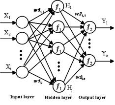
B. Multi Layer Perceptron:

Multi layer perceptron is used for non linear classification. It provides increasing on computational power. The network consist of a set of sensory units, minimum one hidden layer and an output layer. The input signal propagates through the network in a forward direction layer by layer. In multi layer perceptron network receives the signals to get the output. Signal moves in forward direction till getting the output.

Architecture of Multilayer Perceptron:

Back Propagation Algorithm-

Step 1- Initialize weights W,V

Step 2- Submit pattern x and compute layer’s response

Y=Ө[VX]

O=Ө[WY]

Step 3- compute cycle error

E=E+ ½(dK-oK)2

Step 4- calculate [∆W]=µ[y][α]

[∆V]=µ[x][α’]

Step 5- Adjust weights of output layer W(t+1)=W(t)+∆W

Step 6- Adjust  weights of hidden layer V(t+1)=V(t)+∆V

Step 7- check whether more patterns in the training set- If yes, then begin of a new training step and go to step 2. If no, then go to step 8

Step 8- test E<Emax

If false, then set E=0 and begin new training cycle and go to step 2

If true, then stop.

Here α=(dK-oK)oK(1-oK)

Capabilities of neural network such as functional approximation, generalization is due to nonlinear activation function of each neuron. Generalization  means that a trained net could classify data from the same class as the learning data that it has never seen before.

Network purning techniques-

Purning techniques(NONECS, NENECS, NENEPS) can significantly reduce multi layer perceptrons network size and improve network performance in the sense of generalization error.

In NONECS, the absolute error is used as a error measure to reduce the impact of large deviations.

The NENECS(Neuron Error Network Error Correlation Saliency) is defined as the correlation of neuron error and network error.

The NENEPS(Neuron Error Network Error Polynomial Saliency) is based on a regression analysis.

Related Questions and Answers:

Q1. What is adaptive filteration?

Ans.- Automatic removing of errors is called adaptive filteration. Its operation is based on filtering process and adaptive process, which are continuous processes.

Q2. Name the unconstrained optimization methods  used?

Ans.- They are as follows-method of steepest descent, newton’s method, gauss-newton method.

Q3. What are characteristics of linear least square filter?

Ans.- Characteristics are- Filter is built around linear single neuron. Filter is designed using cost function which consists of sum of error squares.

Q4. What is limitation of LMS algorithm?

Ans.- LMS algorithm has slow rate of convergence and is sensitive to input variation and these are the limitation of this algorithm.

Readers can give their suggestions / feedbacks in the given below comment section to improve the article.

Related Topics:

Introduction To Artificial Intelligence

ARTIFICIAL NEURAL NETWORK

Dynamically Driven Recurrent Networks

Back propagation algorithm

back propagation algorithmconvergence theoremperceptronssample questions on perceptron

« Different types of Neural Network with its Architecture Designing a Questionaire and its Types »